Discrete Distributions - Part 1
Contents
A probability distribution of a random variable refers to the probabilities that the random variable takes various values. In the case that the random variable can take only countably many different values, it is called a discrete random variable. In this case, we can summarize the distribution by simply specifying the probabilities of the different values. In this post, we first look at a simple example to get an intuitive idea of distribution of discrete random variable, then talk about some related concepts such as conditional probability, independence of events and random variables, expected value and variance.
Discrete Random Variable
We first use a simple example to explain some probability concepts.
Simple Example: A Weird Dice
Suppose we have a weird dice, let \(X\) be the random variable of the value of the dice when thrown, where the probabilities of getting different values are as follows:
| \(X\) | 1 | 2 | 3 | 4 | 5 | 6 |
|---|---|---|---|---|---|---|
| \(P(X)\) | 0.2 | 0.05 | 0.1 | 0.4 | 0.1 | 0.15 |
Note that the probabilities are all non-negative, and sum to 1. Also note that we have not explicitly specified the sample space, which in practice is usually omitted, as there could be many possible sample spaces, and that when looking at one random variable, the sample space is not very useful anyway. In this case, we could simply regard the set of possible values of the random variable as the sample space, and the random variable is simply the identity function on the sample space. E.g. we could take \(\{1, 2, 3, 4, 5, 6\}\) as the sample space for \(X\) above.
We may visualize the distribution as follows:
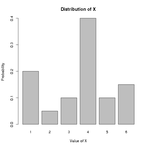
Recall that the probability of an event is the relative frequency of the event when the number of trials approaches infinity. Therefore, if we throw the above weird dice a huge number of times, and plot the bar chart of the proportion of the different values observed, we would get a plot very close to the above.
In this example, the probability of \(X=1\) is twice the probability of \(X=3\), so in a large number of trials (e.g. 10000), we would expect to see about twice as many 1’s as 3’s. The probabilities describe how the trials would be distributed among the different possible values.
With the summation rule of exclusive (also called disjoint) events, we can calculate the probabilities of various events on \(X\).
For example:
| Event | Probability |
|---|---|
| \(X\) is even | \(P(X \in \{2, 4, 6\}) = P(X=2) + P(X=4) + P(X=6)\), which is 0.05 + 0.4 + 0.15 = 0.6 |
| \(X\) is prime | \(P(X \in \{2, 3, 5\}) = P(X=2) + P(X=3) + P(X=5)\), which is 0.05 + 0.1 + 0.1 = 0.25 |
| \(X = 3.5\) | \(P(X = 3.5) = 0\) |
In principle, for any event, we can determine the probability by summing over the appropriate probabilities.
Probability Mass Function
In general, to summarize the distribution of a discrete random variables, we only need to specify its probabilities on different values. The function \(f_X(x) = P(X=x)\) is called the Probability Mass Function (pmf for short) of the discrete random variable \(X\).
Probability values are non-negative and no larger than 1, and that the probability of a sure event is 1. Therefore, for the random variable \(X\) in the dice example, any sequence of 6 non-negative numbers that sum to 1 could specify a possible distribution.
If a random variable can take only a finite number of values, it is possible to explicitly list the probabilities of the different values, as we have done in the above example. On the other hand, when a random variable can take infinitely many different values, it is impossible to explicitly list out the probabilities, therefore a formula is used for the Probability Mass Function. In fact, often it is more convenient to use a formula even for the finite case. The formula often has (usually a small number) parameters that let us vary values of the probability, and the parameters often have interpretation in the situation being modeled. Such distributions are called parametric distributions. We will see concrete examples later in a future post, but before that, let’s talk about some useful basic concepts.
Conditional Probability and Bayes Rule
If we know partial information on the value of a random variable, but not its exact value, will the probabilities of the different values change? In the weird dice example, can we make sense of sentence such as “what is the probability that \(X\) is 4, given that it is even”?
In the frequentist interpretation, a probability is the relative frequency of an event in infinitely many trials. Then it seems reasonable to interpret the above sentence as “the relative frequency of 4 among the trials that are even, in an infinitely many trials”. Let’s say we throw the dice 10,000 times, we would expect the approximate number of times of the different values as follows:
| \(X\) | 1 | 2 | 3 | 4 | 5 | 6 |
|---|---|---|---|---|---|---|
| \(P(X)\) | 0.2 | 0.05 | 0.1 | 0.4 | 0.1 | 0.15 |
| approx. frequency in 10,000 throws | 2000 | 500 | 1000 | 4000 | 1000 | 1500 |
| relative frequency among even throws | 0 | 500/6000 | 0 | 4000/6000 | 0 | 1500/6000 |
| approx. frequency in \(n\) throws | \(0.2n\) | \(0.05n\) | \(0.1n\) | \(0.4n\) | \(0.1n\) | \(0.15n\) |
| relative frequency among even throws | 0 | 0.05 / 0.6 | 0 | 0.4 / 0.6 | 0 | 0.15 / 0.6 |
Out of 10,000 throws, approximately 500 + 4000 + 1500 = 6000 throws would be even, therefore, among these throws, the relative frequency of 4 is 4000/6000 = 2/3. We note that the number “10,000” does not play a crucial role. If we consider \(n\) throws, approximately \(0.05n + 0.4n + 0.15n\) would be even, and the relative frequency of 4 among even throws would be approximately \(\frac{0.4n}{0.6n} = \frac{2}{3}\), where the \(n\) gets cancelled. As \(n\) approaches infinitely, the true relative frequency should converge to \(\frac{2}{3}\), which is \(\frac{P(X=4)}{P(X \text{ is even})}\).
In the Bayesian interpretation, probability is a degree of belief of an event, normalized such that the degree of belief of the sure event is 1. Before knowing anything about the value of the dice throw, our degree of belief that it is 4 would be \(P(X=4) = 0.4\), and that it is 3 is \(P(X=3) = 0.1\), which means we believe it is 4 times more likely to get a 4 as opposed to a 3. Having learnt that the throw is even, our degree of belief should be updated, in particular, now the only possibilities are 2, 4 or 6, therefore we know that it cannot be 3, so the degree of belief that “it is 3 given that it is even” would be 0. Intuitively, out of the possibilities 2, 4, and 6, we need only figure out their relative degree of belief, to again get a normalized degree of belief. Note that dividing the degree of belief by the same number would not change their relative degree of belief, so we need only divide them by a number \(c\) such that they sum to 1. A moment of thought would reveal that we should divide by
\begin{equation}
c = P(X \text{ is even}) \\\
= P(X=2) + P(X=4) + P(X=6)
\end{equation}
because then their sum would be
\begin{equation}
\frac{P(X=2)}{c} + \frac{P(X=4)}{c} + \frac{P(X=6)}{c} \\\
\text{ which is } \\\
\frac{P(X=2) + P(X=4) + P(X=6)}{c} = 1 \text{ as desired.}
\end{equation}
Therefore, the “the probability that \(X\) is 4, given that it is even” would be \(\frac{P(X=4)}{P(X \text{ is even})}\), which is \(\frac{0.4}{0.6} = \frac{2}{3}\), and unsurprisingly the same as the value above.
The concept such as “the probability that \(X\) is 4, given that it is even” is called conditional probability. In general, “the probability of event A, given the event B”, denoted as \(P(A|B)\) is defined as
\begin{equation} P(A|B) = \frac{P(A \text{ and } B)}{P(B)} \end{equation}
where it is assumed that \(P(B) > 0\).
We can visualize it as follows:
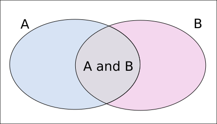
Where the rectangle represents the sample space with area 1, and the two ovals represent the events A and B, and their areas are the respective probabilities of event A and B. When given event B, the possibilities are reduced from the rectangle to the oval B, and to determine “the probability of A, given B”, i.e. \(P(A|B)\), we only need to figure out the relative ratio of area of “A and B” (the grey part) to “(not A) and B” (the pink part), and normalize them to sum to 1. Since the areas of “A and B” and “(not A) and B” sums to the area of “B”, therefore \(P(A|B)\) would be \(\frac{P(A \text{ and } B)}{P(B)}\).
Moreover, by rearranging the terms of \(P(A|B) = \frac{P(A \text{ and } B)}{P(B)}\), we have
\begin{equation} P(A \text{ and } B) = P(B)P(A|B) \end{equation}
and similarly we also have
\begin{equation} P(A \text{ and } B) = P(A)P(B|A) \end{equation}
where we can decompose \(P(A \text{ and } B)\) into two parts, which sometimes may be easier to compute.
We also briefly mention the famous Bayes rule, which is a direct consequence of the definition of conditional probability:
\begin{equation}
P(A|B) = \frac{P(A \text{ and } B)}{P(B)} \\\
= \frac{P(A)P(B|A)}{P(B)}
\end{equation}
which is very useful when determining \(P(B|A)\) is easier than determining \(P(A|B)\). An example of application of the Bayes rule is the naive Bayes classifier, but we will not go into details here.
Independence:
Independent Events
Independence is a very important concept in probability, as it often simplifies a lot of calculations. Let’s start with independent events. What does it mean to say “event A is independent of event B”? One reasonable idea is that “knowing B does not give additional useful information about A, and vice versa”, in other words, “knowing B does not change the probability of A”. In the language of conditional probability, this would mean that \(P(A|B) = P(A)\) and \(P(B|A) = P(B)\).
Recall that we have \(P(A \text{ and } B) = P(A)P(B|A)\), so that if A and B are independent (accordingly to our intuitive idea above), we would have \(P(A \text{ and } B) = P(A)P(B)\). On the other hand, if we have \(P(A \text{ and } B) = P(A)P(B)\), we then have
\begin{equation}
P(A|B) = \frac{P(A \text{ and } B)}{P(B)} \\\
= \frac{P(A)P(B)}{P(B)} \\\
= P(A)
\end{equation}
And similarly we get \(P(B|A) = P(B)\). We therefore see that these two conditions are essentially equivalent, but \(P(A \text{ and } B) = P(A)P(B)\) is usually taken as the definition of “A and B are independent events”, because it is also well defined when either \(P(A)\) or \(P(B)\) is zero.
For more than two events, you can probably guess how the definition for two events should be extended:
A set of \(k\) events \(A_k\) are mutually independent if and only if
\begin{equation} P(A_1 \text{ and } A_2 \text{ and } \ldots \text{ and } A_k) \\\
= P(A_1)P(A_2)\ldots P(A_k) \end{equation}
We can two visualize independent events as follows:
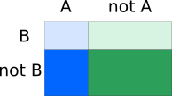
where the four regions with different colours represent different combinations of whether event A and B have occurred. Note that the areas align very well such that given B (restricting to the areas in the top row), the ratio of area of A to “not A” has not changed.
On the other hand, for dependent events, to more clearly illustrate, we exaggerate in the following diagram.
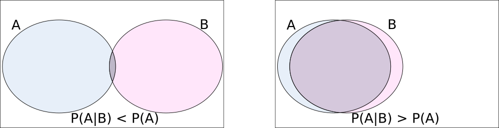
Note that \(P(A)\) and \(P(B)\) have not changed in the two pictures, but it is clear that on the left, \(P(A|B) < P(A)\), whereas on the right, \(P(A|B) > P(A)\).
In the above weird dice example, we have already seen a pair of dependent events: “the number is even” and “the number is 4”. For the weird dice example, it is difficult to find independent events, but we can see examples of independent events when we discuss independent random variables below.
Independent Random Variables
Suppose that I throw the weird dice above, and my friend flips a biased coin, would we expect the outcomes of the dice and the coin to be dependent? I guess not. But what would it mean to say the two random variables are independent? In the same spirit of two independent events, we may consider along the line of “knowing the value of one random variable does not give additional useful information about the other random variable, and vice versa”. For a random variable, the useful information is its probability distribution, so we may rephrase this idea of independent random variables as “given the value of one random variable, the probability distribution of the other is not changed, and vice versa”.
We have already seen the probability distribution of the value of the dice \(X\) above, we copy it to here for convenience.
| \(X\) | 1 | 2 | 3 | 4 | 5 | 6 |
|---|---|---|---|---|---|---|
| \(P(X)\) | 0.2 | 0.05 | 0.1 | 0.4 | 0.1 | 0.15 |
Just for concreteness, suppose the distribution of the biased coin \(Y\) is
| \(Y\) | H | T |
|---|---|---|
| \(P(Y)\) | 0.3 | 0.7 |
If \(X\) and \(Y\) are independent, what should be the probability distribution of the pair \((X, Y)\)? If knowing \(Y\) does not change our belief on the probabilities of \(X\), then for any values \(x\) and \(y\), we should have: \(P(X=x|Y=y) = P(X=x)\). But since
\begin{equation} P(X=x|Y=y) = \frac{P(X=x, Y=y)}{P(Y=y)} \end{equation}
we see that we should have \(P(X=x, Y=y)\) = \(P(X=x)P(Y=y)\), the similar form of multiplication of probabilities as in independent events!
Therefore, the distribution of \(X\) and \(Y\) together (called the joint distribution) would look like this:
| \(X=1\) | \(X=2\) | \(X=3\) | \(X=4\) | \(X=5\) | \(X=6\) | \(P(Y)\) | |
|---|---|---|---|---|---|---|---|
| \(Y=H\) | 0.06 | 0.015 | 0.03 | 0.12 | 0.03 | 0.045 | 0.3 |
| \(Y=T\) | 0.14 | 0.035 | 0.07 | 0.28 | 0.07 | 0.105 | 0.7 |
| \(P(X)\) | 0.2 | 0.05 | 0.1 | 0.4 | 0.1 | 0.15 |
You may try to verify that indeed we have \(P(X=x,Y=y)\) = \(P(X=x)P(Y=y)\). Note that in the joint distribution of \(X\) and \(Y\), the sums of each row give the probability distribution of \(Y\), and the sums of each column give the probability distribution of \(X\). When two or more random variables are defined on the same sample space, the distribution of them together is called the joint distribution, and the distribution of one random variable alone is called the marginal distribution. The marginal distribution can be obtained by summing (in the discrete case) over all the possible values of other random variables in the joint distribution (a process called marginalization).
In fact independence of random variable is defined as:
Two random variables \(X\) and \(Y\) are independent if and only if
\(P(X \in A \text{ and } Y \in B) = P(X \in A)P(Y \in B)\) for any events \(\{X \in A\}\) and \(\{Y \in B\}\).
This definition implies the condition we considered above, by taking the events be \(X=x\) and \(Y=y\). And for discrete random variables, it is easy to see the above condition implies the definition here, because the probability of any event can be calculated from the appropriate sums. Indeed, suppose \(A=\{x_1, x_2, \ldots\}\) and \(B=\{y_1, y_2, \ldots\}\), we have
\begin{equation}
P(X \in A \text{ and } Y \in B) = \sum_i\sum_j{P(X=x_i, Y=y_j)} \\\
= \sum_i\sum_j{P(X=x_i)P(Y=y_j)} \\\
= \left\{\sum_i{P(X=x_i)}\right\} \left\{\sum_j{P(Y=y_j)}\right\} \\\
= P(X \in A)P(Y \in B)
\end{equation}
You may have already guessed the definition of independence of \(k\) random variables. In fact, we can extend the definition to countably many random variables:
A sequence of random variables \(\{X_1, X_2, \ldots\}\) are mutually independent if and only if for any finite subset of them (no duplicates), say \(\{X_{s_1}, X_{s_2}, \ldots, X_{s_k}\}\), we have
\begin{equation} P(X_{s_1} \in A_{s_1}, X_{s_2} \in A_{s_2}, \ldots, X_{s_k} \in A_{s_k}) = \\\
P(X_{s_1} \in A_{s_1})P(X_{s_2} \in A_{s_2})\ldots P(X_{s_k} \in A_{s_k}) \end{equation}for any events \(\{X_{s_i} \in A_{s_i}\}\).
Expected Value and Variance
Basic idea of expected value
For numeric random variable (but we would only consider real-valued random variables), we can define some sort of “average” for it. Since each value may have different probabilities, intuitively we should weight by the probabilities. This intuition is exactly the definition of expected value of a discrete random variable.
The expected value of a discrete random variable \(X\), denoted as \(E(X)\) is defined as
\begin{equation} E(X) = \sum_i{x_i P(X=x_i)} \end{equation}
For the weird dice above, we can calculate the expected value of \(X\) as
|
|
|
|
If we throw the weird dice a large number of times (say 10,000), and then take the arithmetic mean of the realized values, we should obtain a number very close to the expected value 3.6, because the proportion that each value appears is close to the probability. In general, for a discrete numeric random variable, the arithmetic mean of a large number of independent trials will converge to the expected value, as the number of trials approaches infinity.
We note that the expected value is not an integer, and is not a possible value of \(X\). This is often the case for discrete random variable, which are usually integer valued. The expected value is also called the mean, and could be regarded as some sort of “center” value (another reasonable and usual definition of the “center” is the median).
We not only can take the “average” of the random variable itself, but in fact functions of the random variable.
The expected value of a function \(g\) on a discrete random variable \(X\), denoted as \(E(g(X))\) is defined as
\begin{equation} E(g(X)) = \sum_i{g(x_i) P(X=x_i)} \end{equation}
For example, for the weird dice, we may calculate \(E(X^2)\)
|
|
|
|
In particular, the expected value of a constant \(a\) is the constant itself, i.e. \(E(a)\) = \(\sum_i{a P(X=x_i)}\) = \(a \sum_i{ P(X=x_i)}\) = \(a (1)\) = \(a\).
Recall that a random variable \(X\) is a function on the sample space, so \(g(X)\) is also a function on the sample space, which means \(g(X)\) is also a random variable.
We can also calculate the expected value of (numeric) functions of two or more (not necessarily independent) random variables (defined on the same probability space). For example, if we have two discrete random variables \(X_1\) and \(X_2\) defined on the same probability space, then \(E(X_1 + X_2)\) is well defined, which is summing \(x_1 + x_2\) over all the possible combinations of \(X_1=x_1\) and \(X_2=x_2\) weighted by \(P(X_1=x_1, X_2=x_2)\). Similarly, \(E(X_1 X_2)\) is also well defined, which is summing \(x_1 x_2\) over all the possible combinations of \(X_1=x_1\) and \(X_2=x_2\) weighted by \(P(X_1=x_1, X_2=x_2)\). The expected value \(E(g(X_1, X_2))\) is calculated similarly for a function \(g\).
Some properties of expected value
We just briefly mention a very nice property of expected value: linearity, which means
\begin{equation}
E(a_1 X_1 + a_2 X_2 + \ldots + a_k X_k) = \\\
a_1 E(X_1) + a_2 E(X_2) + \ldots + a_k E(X_k)
\end{equation}
where the \(\{a_i\}\) are constants, and the random variables \(\{X_i\}\) are not necessarily independent. In words, if a random variable is scaled by a constant, its expected value is also scaled by the same constant; and the expected value of a sum of random variables is just the sum of the expected values of the random variables. For example, we have \(E(X + 3 X^2) = E(X) + 3E(X^2)\), even though \(X\) and \(X^2\) are dependent random variables.
But it is important to note that \(E(X_1 X_2)\) does not necessarily equal \(E(X_1)E(X_2)\). For example, for the weird dice, \(E(XX) = E(X^2) = 15.6\) as calculated above, and \(E(X)E(X)\) = \((3.6)(3.6)\) = 12.96. However, if \(X_1\) and \(X_2\) are independent random variables, we indeed would have \(E(X_1 X_2)\) = \(E(X_1) E(X_2)\).
Variance: expected squared deviation from the mean
We mentioned expected value of a random variable is some sort of “center”, can we have a measure of how “spreaded out” (i.e. the dispersion of) the distribution of the random variable is? One idea is to calculate the “average” of the deviation from the “center”. One such measure is the variance, denoted by \(Var(X)\), and is defined as:
The variance of a numeric random variable \(X\) is defined as
\(Var(X) = E(X - \mu)^2\), where \(\mu = E(X)\).
Note that for a given random variable \(X\), its mean \(E(X)\) is a constant (we usually use the letter \(\mu\) for mean), so the variance is the expected value of squared difference from the mean. There are other measures of dispersion which do not take the average of squared deviation, but rather the average of absolute deviation, but we would not discuss these here.
It is intuitively clear that a random variable with a more concentrated distribution has less variation, and therefore a smaller variance, as illustrated in the following plots:
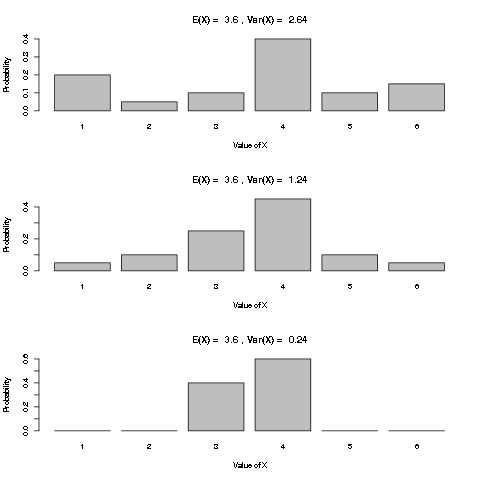
With \(\mu = E(X)\), and the properties of expected value, we see that
\begin{equation}
Var(X) = E(X - \mu)^2 \\\
= E(X^2 - 2\mu X + \mu^2) \\\
= E(X^2) - E(2\mu X) + E(\mu^2) \\\
= E(X^2) - 2 \mu E(X) + \mu^2 \\\
= E(X^2) - 2 \mu \mu + \mu^2 \\\
= E(X^2) - \mu^2 \\\
= E(X^2) - [E(X)]^2 \\\
\end{equation}
which gives an alternative formula to calculate the variance.
If the random variable has units (e.g. kg), the unit of its variance would also be squared (e.g. kg squared), and therefore does not have the same scale as the random variable. To remedy this, we take the square root of the variance, which is called the standard deviation of the random variable \(X\), often denoted with the letter \(\sigma\), as in \(\sigma_X = \sqrt{Var(X)}\).
Summary
In this post, we have looked at the concepts related to the distribution of a discrete random variable through some simple examples:
- discrete random variable: a random variable with at most countably many different values.
- probability mass function: \(f_X(x) = P(X=x)\), the function giving the probabilities for different values of a discrete random variable.
- conditional probability: \(P(A|B)\), the probability of an event \(A\), given that another event \(B\) has occurred.
- independent events: events \(A\) and \(B\) are independent if \(P(A \text{ and } B) = P(A)P(B)\).
- independent random variables: two random variables are independent if \(P(X \in A \text{ and } Y \in B) = P(X \in A)P(Y \in B)\) for any events \(\{X \in A\}\) and \(\{Y \in B\}\).
- expected value of discrete numeric random variable: sum of the possible values of the random variable, weighted by the probabilities of the values.
- variance of discrete numeric random variable: expected value of squared deviation from the mean of random variable.
We will look at some common examples of discrete random variables in a future post, before we turn to look at continuous random variables.
Author Peter Lo
LastMod 2019-05-27