Discrete Distributions - Part 2
Contents
In the previous post, we have looked at some basic concepts of distributions of discrete random variable. In this post we look at some examples of common discrete random variables, including discrete uniform distribution, Bernoulli distribution, Binomial distribution, Geometric distribution, Negative binomial distribution and Poisson distribution.
Common Discrete Distributions
Discrete Uniform Distribution
When a discrete random variable has \(k\) different possible values, and we think that the different possibilities are equally likely, what should the distribution be? Since the \(k\) equal probabilities should sum to 1, it follows that each probability should be \(\frac{1}{k}\). This is the discrete uniform distribution, with the parameter \(k\), the number of possibilities. This distribution is often used to model situations where either we believe that the possibilities are equally likely, e.g. due to symmetry; or we lack more specific information to believe that they should be different, so can only assume that they are equally likely.
Note that we cannot have discrete uniform distribution with infinitely many possible values, because the probabilities have to be equal in a uniform distribution, but also need to sum to 1. We just briefly mention that it is possible to have continuous uniform distribution with infinitely many different possible values, but its range still has to be bounded.
Fair coin and dice
For example, for a coin that we know little about, we only know that it is fairly symmetric, so we have no reason to think that one side is more likely to come up than the other side. Even if we suspect that the coin is biased, how do we know which side would come up more often, without observing at least some trials? In such case, it is quite reasonable to assume the probabilities of both sides to be at top when flipped to be \(\frac{1}{2}\), ignoring the possibility that it may land on the edge.
As another example, for a regular dice with 6 faces, since it is mostly symmetric, it is reasonable to assume uniform distribution, i.e. a probability of \(\frac{1}{6}\) for each face.
Random ordering
Yet another example is random ordering or random permutation. For \(n\) objects, there are \(n! = n \times (n-1) \times \ldots \times 2 \times 1\) different ordering (permutation). For example, for 3 objects \(\{A, B, C\}\), there are \(3! = 3 \times 2 \times 1 = 6\) different orderings:
| 1st | 2nd | 3rd |
|---|---|---|
| A | B | C |
| A | C | B |
| B | A | C |
| B | C | A |
| C | A | B |
| C | B | A |
Because in the first position, we have 3 choices, then once that is selected, for the second position, we have 2 choices remaining, and once that is also selected, we have only one choice for the third position. In general, for \(n\) objects, we have \(n\) choices for the first position, then once it is selected, we have \(n-1\) choices for the second position, then \(n-2\) for the third, and so on, until we get down to only one choice for the last position; therefore the number of different orderings for \(n\) objects is the formula above, denoted by \(n!\) (pronounced as “n factorial”). For a deck of 52 cards, the number of ordering is \(52!\), which is a huge number: 80658175170943878571660636856403766975289505440883277824000000000000.
What should be the probability of each of the \(n!\) possible orderings, if we want a uniform distribution? From our previous discussion, the answer is obvious: each should have probability \(\frac{1}{n!}\). As a digression, sometimes we have some bias against some “patterns”, even though we meant to have a uniformly random ordering. For example, if we were to get a random ordering of the integers 1 to 5 (by a supposedly uniform method), and the ordering turn out to be (1, 2, 3, 4, 5) or (5, 4, 3, 2, 1), some people may suggest that this is not random enough, and therefore should be re-shuffled to get a more random ordering, such as (2, 1, 4, 3, 5). But if we think about it, by biasing against some “patterns” and re-shuffle when they occur, even if the original random ordering process is uniform, the ordering (1, 2, 3, 4, 5) has a lower chance of being selected and therefore the distribution would be non-uniform! To get a uniformly random ordering, we need a uniformly random selection process, not look at the selected ordering. And as an interesting thought experiment, imagine switching the integers 1 to 5 to five distinct symbols unfamiliar to us, would we still bias against some “patterns”?
Expected value
If the discrete uniformly distributed random variable is real-valued, we can calculate its expected value and variance. For example, if the possible values are the integers 1, 2, 3, 4, 5 and 6, then the expected value is
|
|
|
|
And the variance would be
|
|
|
|
If the possible values are 1, 236 and 12, then the expected value would be
|
|
|
|
And the variance would be
|
|
|
|
Bernoulli Distribution
One particularly simple discrete distribution is that of an indicator variable which can only take the values 0 or 1. The distribution is called the Bernoulli distribution, where the probability of 1 is \(p\), and the probability of 0 is \(1-p\), and \(0 \leq p \leq 1\) is the parameter of the distribution. Note that the case of \(p=0\) or \(p=1\) is degenerate case, because then the random variable is really just a constant. That a random variable \(X\) follows a Bernoulli distribution with parameter \(p\) is sometimes written as \(X \sim \text{Bernoulli}(p)\). It should be emphasized that different values of the parameter \(p\) give different Bernoulli distributions, although they have similar form. So Bernoulli distribution is really a family of distributions with similar form, and the parameter identifies a particular member of the family.
The Bernoulli distribution is used to model whether an event has occurred, e.g. “the coin lands on head”, “the dice has the value 6”, or binary outcomes such as “yes/no”, “success/failure”, “has disease/no disease” cases. The interpretation of the Bernoulli distribution is the count of occurrence of event, but with just one trial.
Although we would often assign the value 1 to “yes” in “yes/no”, to “success” in “success/failure” situation, we emphasize that it is important to define clearly the event for which the random variable takes the value 1, because in binary outcomes, there may not be a “natural” choice, or that choice may depend on context. For example, we may define “has disease” as the event, thus takes value 1, but we may also think that “no disease” is a success, thus should take the value 1. Therefore it is a better idea to be explicit.
Note that if a random variable \(X\) has Bernoulli distribution with parameter \(p\), \(1-X\) (clearly \(X\) and \(1-X\) are dependent) is also a random variable with Bernoulli distribution, but with parameter \(1-p\). When the parameter \(p\) is \(0.5\), the outcomes 0 and 1 are equally likely, and the distribution is uniform.
Expected value and variance
With only two possible outcomes, it is easy to calculate the expected value of a random variable \(X\) having Bernoulli distribution with parameter \(p\):
\begin{equation} E(X) = 1 \times p + 0 \times (1 - p) = p \end{equation}
Calculating the variance is equally straightforward:
\begin{align}
Var(X) & = E[(X - [E(X)])^2] \\\
& = (1 - p)^2 \times p + (0 - p)^2 \times (1 - p) \\\
& = p(1 - p)^2 + p^2(1-p) \\\
& = p(1 - p)[1 - p + p] \\\
& = p(1 - p)
\end{align}
Note that since \(0 \leq p \leq 1\), we can plot the variance with different values of \(p\):
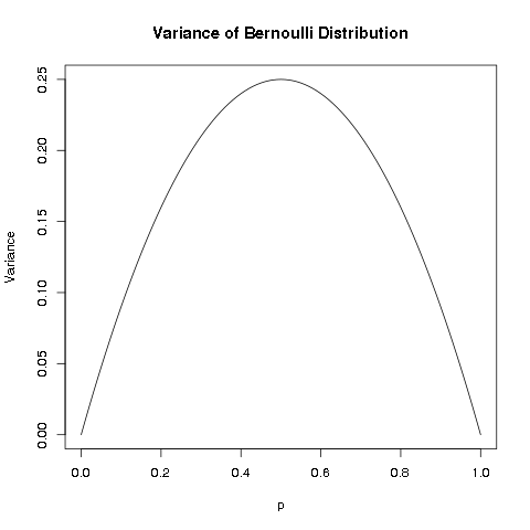
We can see that the variance is 0 at the two ends \(p=0\) and \(p=1\), because for these two degenerate cases, the random variable becomes a constant, and therefore has no “variation”. As the parameter \(p\) is further from the two ends, the variance increases, but is bounded. From the plot and the symmetry of \(p(1-p)\), we can easily reason that the maximum occurs at the middle, i.e. at \(p=0.5\). We can also use either calculus or a little algebra, to determine that the variance is maximum at \(p=0.5\). Therefore, the maximum possible variance of Bernoulli distribution is 0.25.
Binomial Distribution
While the Bernoulli distribution counts the number of events in one trial, how about more trials? For example, if I flip a coin 10 times, and count the number of heads, what should the distribution of the count be? Let’s say \(X_1 \sim \text{Bernoulli}(p)\) is the indicator for “head” in the first flip. Since we are considering repeatedly flipping the same coin 10 times, so let \(X_i \sim \text{Bernoulli}(p)\) be the indicator for “head” in the \(i\) th flip, i.e. the 10 random variables \(\{X_i: 1 \leq i \leq 10\}\) are identically distributed (have the same distribution). Moreover, it is reasonable to assume that the different flips are independent. In this case, we say the 10 random variables \(\{X_i: 1 \leq i \leq 10\}\) are independent identically distributed, or i.i.d. for short. Then what we are interested in is the distribution of the random variable \(X = X_1 + X_2 + \ldots + X_{10}\). The distribution of a sum of \(n\) i.i.d. random variables with Bernoulli distribution (with parameter \(p\)) is called the Binomial distribution, written as \(B(n, p)\). When \(n=1\), it reduces to a Bernoulli distribution. It is obvious that if \(X \sim B(n,p)\), then \(0 \leq X \leq n\), i.e. the smallest possible count is 0, and the largest possible count is \(n\).
Probability mass function for Binomial distribution
If \(X \sim B(n,p)\), since the only way to get \(X=n\) is to have all the \(X_i=1\), we quickly see that:
\begin{align}
P(X=n) & = P(X_1=1, X_2=1, \ldots, X_n=1) \\\
& = P(X_1=1)P(X_2=1)\ldots P(X_n=1) \\\
& = p^n
\end{align}
Similarly, we have \(P(X=0) = (1-p)^n\) because the only way to get \(X=0\) is to have all the \(X_i=0\). Let’s see more examples before figuring out the general formula of the probability mass function of Binomial distribution.
Consider \(Y \sim B(5, p)\), to find \(P(Y = 1)\), we want the probability of 1 success and thus (5-1=4) failures. We list out the possible ways of getting one success:
| Trial 1 | Trial 2 | Trial 3 | Trial 4 | Trial 5 | Probability |
|---|---|---|---|---|---|
| 1 | 0 | 0 | 0 | 0 | \(p(1-p)(1-p)(1-p)(1-p) = p(1-p)^4\) |
| 0 | 1 | 0 | 0 | 0 | \((1-p)p(1-p)(1-p)(1-p) = p(1-p)^4\) |
| 0 | 0 | 1 | 0 | 0 | \((1-p)(1-p)p(1-p)(1-p) = p(1-p)^4\) |
| 0 | 0 | 0 | 1 | 0 | \((1-p)(1-p)(1-p)p(1-p) = p(1-p)^4\) |
| 0 | 0 | 0 | 0 | 1 | \((1-p)(1-p)(1-p)(1-p)p = p(1-p)^4\) |
We first notice that for each combination of 1 success and 4 failures, the probability is the same: \(p(1-p)^4\), so it suffices to count the number of combinations to get the proper sum. We see that there are 5 possible positions where the 1 success may come from, and there are exactly 5 combinations. Therefore \(P(Y=1) = 5p(1-p)^4\).
Let’s also figure out \(P(Y = 2)\), we want the probability of 2 successes and thus (5-2=3) failures. But the 2 successes may be from the different trials, as illustrated below:
| Trial 1 | Trial 2 | Trial 3 | Trial 4 | Trial 5 | Probability |
|---|---|---|---|---|---|
| 1 | 1 | 0 | 0 | 0 | \(pp(1-p)(1-p)(1-p) = p^2(1-p)^3\) |
| 1 | 0 | 1 | 0 | 0 | \(p(1-p)p(1-p)(1-p) = p^2(1-p)^3\) |
| 1 | 0 | 0 | 1 | 0 | \(p(1-p)(1-p)p(1-p) = p^2(1-p)^3\) |
| 1 | 0 | 0 | 0 | 1 | \(p(1-p)(1-p)(1-p)p = p^2(1-p)^3\) |
| 0 | 1 | 1 | 0 | 0 | \((1-p)pp(1-p)(1-p) = p^2(1-p)^3\) |
| 0 | 1 | 0 | 1 | 0 | \((1-p)p(1-p)p(1-p) = p^2(1-p)^3\) |
| 0 | 1 | 0 | 0 | 1 | \((1-p)p(1-p)(1-p)p = p^2(1-p)^3\) |
| 0 | 0 | 1 | 1 | 0 | \((1-p)(1-p)pp(1-p) = p^2(1-p)^3\) |
| 0 | 0 | 1 | 0 | 1 | \((1-p)(1-p)p(1-p)p = p^2(1-p)^3\) |
| 0 | 0 | 0 | 1 | 1 | \((1-p)(1-p)(1-p)pp = p^2(1-p)^3\) |
Again we see that for each combination of 2 successes and 3 failures, the probability is the same value \(p^2(1-p)^3\), so it suffices to count the number of combinations to get the proper sum. As there are 5 possible positions where the 2 successes may come from, and there are 10 combinations. Therefore \(P(X_1 = 2) = 10{p^2(1-p)^3}\).
It is easy to see that we can use the same reasoning to derive the probability of \(P(X=r)\), where \(X \sim B(n,p)\): we want the probability of \(r\) successes (i.e. \(n-r\) failures), but the \(r\) successes may come from the \(n\) different trials, each combination has the same probability of \(p^r(1-p)^{n-r}\) for \(r\) successes and \(n-r\) failures. We only need to figure out the number of combinations that \(r\) successes can appear in \(n\) trials. The number of combinations of choosing \(r\) distinct objects from \(n\) distinct objects, disregarding the order, is called the Binomial coefficient, denoted by \(C_r^n\) (note that some people would write \(_n C_r\) or \(C_n^r\) for what we write \(C_r^n\)) or \({n \choose r}\), pronounced as “\(n\) choose \(r\)”.
Therefore the probability mass function for \(X \sim B(n,p)\) is
\begin{equation} P(X=r) = C_r^n p^r (1-p)^{n-r} \end{equation}
Formula of n choose r
The formula for \(C_r^n\) is
\begin{equation} C_r^n = \frac{n!}{r!(n-r)!} \end{equation}
where \(n! = n \times (n-1) \times (n-2) \times \ldots \times 1\) is \(n\) factorial (recall that it is the number of permutations of n objects).
To get an idea of the formula of \(C_r^n\), consider \(C_2^5\), i.e. how many ways of choosing 2 distinct objects from 5 distinct objects (say {A, B, C, D, E}), disregarding the order. From the formula, we have \(C_2^5 = \frac{5!}{2!3!} = 10\), the same number we have determined above. Well, let’s follow a similar line of thought in deriving the number of permutations: there are 5 choices for the first one, then 4 choices for the second one, so it would seem the answer is \(5 \times 4 = 20\)? No, this over-counts, because this way of counting treats different ordering as distinct! With this way of counting, the counted combinations are:
| first object | combinations |
|---|---|
| A | {(A, B), (A, C), (A, D), (A, E)} |
| B | {(B, A), (B, C), (B, D), (B, E)} |
| C | {(C, A), (C, B), (C, D), (C, E)} |
| D | {(D, A), (D, B), (D, C), (D, E)} |
| E | {(E, A), (E, B), (E, C), (E, D)} |
The problem is that for every set of 2 objects, we counted twice: e.g. (A, B) and (B, A). Therefore, to get the correct number of \(C_2^5\), we need only account for the over-counting by dividing \(5 \times 4\) by 2, to get \(C_2^5 = \frac{5 \times 4}{2} = 10\). Note that we can also write
\begin{align}
C_2^5 & = \frac{5 \times 4}{2} \\\
& = \frac{5 \times 4 \times 3 \times 2 \times 1}{(2 \times 1)(3 \times 2 \times 1)} \\\
& = \frac{5!}{2!3!}
\end{align}
In general, to count \(C_r^n\), there are \(n\) choices for the first object, \(n-1\) for the second, \(n-2\) for the third, and so on, up to \(n-r+1\) for the \(r\) th object, with \(n \times (n-1) \times (n-2) \times \ldots \times (n-r+1)\) combinations. But again, this over-counts: for each subset of \(r\) objects, all the \(r!\) of its permutations are counted. So we divide by \(r!\) to get
\begin{align}
C_r^n & = \frac{n \times (n-1) \times (n-2) \times \ldots \times (n-r+1)}{r!} \\\
& = \frac{n \times (n-1) \times (n-2) \times \ldots \times (n-r+1) \times (n-r)!}{(n-r)!r!} \\\
& = \frac{n!}{(n-r)!r!}
\end{align}
One interesting property of \(C_r^n\) is that
\begin{equation} C_r^n = C_{n-r}^n \end{equation}
E.g. \(C_2^5 = C_3^5\). This can be understood as: specifying which \(r\) objects to take from \(n\), is the same as specifying which \(n-r\) objects not to take, and therefore the counts are the same.
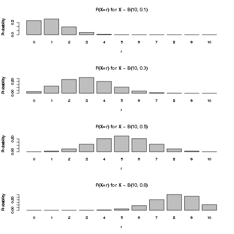
We can plot the pmf of \(B(10, p)\) for a few values of \(p\) to get a better intuitive idea of the Binomial distribution:
Example: number of insurance claims in the next year
As a simple example, suppose we (as an insurance company) have sold \(n\) policies with coverage for the next year. If we assume whether the policies would have claims are reasonably independent, and have the same probability \(p\), then the total number of claims for the coming year would follow a Binomial distribution \(B(n,p)\). Of course, the assumptions of this simple model are quite strong, and it models only the total claims, so would be appropriate in case each policy could make at most one claim in the coming year, and that the payment for each claim is a fixed amount.
Expected value and variance
In order to calculate the expected value of \(X \sim B(n,p)\), we could have used the definition \(E(X) = \sum_{r=0}^n{r P(X=r)}\), but the algebra is more involved.
Instead, we use the fact that \(X\) is the same as a sum of \(n\) i.i.d. random variables following Bernoulli distribution, i.e. \(X = \sum_{i=1}^n{X_i}\), where \(X_i \sim Bernoulli(p)\). Then using the linearity of expected value, we have:
\begin{align}
E(X) & = E(\sum_{i=1}^n{X_i}) \\\
& = \sum_{i=1}^n{E(X_i)} \\\
& = \sum_{i=1}^n{p} \\\
& = np
\end{align}
The expected value is very intuitive, since each of the \(n\) trials has a success probability of \(p\), the expected number of successes is simply \(n \times p\).
For the variance, we first derive the rule that the variance of sum of independent random variables is the sum of the variances. For a sum of \(n\) random variables \(\{X_i\}\), with \(E(X_i) = \mu_i\), we have:
\begin{align}
Var(\sum_{i=1}^n X_i) & = E\{(\sum_{i=1}^n X_i - E(\sum_{i=1}^n X_i))^2\} \\\
& = E\{(\sum_{i=1}^n X_i - \sum_{i=1}^n \mu_i)^2\} \\\
& = E\{(\sum_{i=1}^n (X_i - \mu_i))^2\} \\\
& = E\{\sum_{i=1}^n \sum_{j=1}^n {(X_i - \mu_i)(X_j - \mu_j)} \} \\\
& = E\{\sum_{i=1}^n (X_i - \mu_i)^2 + \sum_{i=1}^n \sum_{j=1, j \neq i}^n {(X_i - \mu_i)(X_j - \mu_j)} \} \\\
& = \sum_{i=1}^n E\{(X_i - \mu_i)^2\} + \sum_{i=1}^n \sum_{j=1, j \neq i}^n E[(X_i - \mu_i)(X_j - \mu_j)] \\\
& = \sum_{i=1}^n Var(X_i) + \sum_{i=1}^n \sum_{j=1, j \neq i}^n Cov(X_i, X_j)
\end{align}
where \(Cov(X_i, X_j) = E[(X_i - \mu_i)(X_j - \mu_j)]\) is called the covariance of \(X_i\) and \(X_j\) (whether \(X_i\) and \(X_j\) are independent or not).
Note that for two independent random variables, we have
\begin{align}
Cov(X_i, X_j) & = E[(X_i - \mu_i)(X_j - \mu_j)] \\\
& = E(X_i - \mu_i) E(X_j - \mu_j) \\\
& = (E(X_i) - \mu_i) (E(X_j) - \mu_j) \\\
& = (\mu_i - \mu_i) (\mu_j - \mu_j) \\\
& = 0
\end{align}
where we use the fact that if \(X_i\) and \(X_j\) are pairwise independent (when \(i \neq j\)), we have \(E(X_i - \mu_i)(X_j - \mu_j) = E(X_i - \mu_i) E(X_j - \mu_j)\), and that both factors would be 0. Therefore the covariance of two independent random variables is 0.
Hence if the random variables \(\{X_i\}\) are pairwise independent, we have:
\begin{equation} Var(\sum_{i=1}^n X_i) = \sum_{i=1}^n Var(X_i) \end{equation}
With this rule of variance for sum of pairwise independent random variables, for \(X \sim B(n,p)\), the variance is
\begin{align}
Var(X) & = Var(\sum_{i=1}^n{X_i}) \\\
& = \sum_{i=1}^n{Var(X_i)} \\\
& = \sum_{i=1}^n{p(1-p)} \\\
& = np(1-p)
\end{align}
Since the variance of the Binomial distribution is essentially just scaled version of the variance of the Bernoulli distribution, the variance is the highest when \(p=0.5\).
Geometric Distribution
If we repeatedly flip a (possibly biased) coin, and we are interested in counting the number of “tails” \(X\) before seeing the first “head” (not including that flip). It is clear that this is a random variable that takes values on non-negative integers, the smallest possible value is 0, but it does not have a theoretical upper bound, i.e. it is conceivable that we are really unlucky that we do not see a “head” in even 1 million flips, although the probability would be exceedingly small (unless the coin is so biased such that it will never land on head). Assuming that each flip giving a “head” follows \(Bernoulli(p)\) with \(0 < p < 1\), and the flips are independent, then this \(X\) follows a Geometric distribution with parameter \(p\). There is an alternative convention that counts the number of trials (instead of the failures) before seeing the first success (having a “head” in this example), i.e. the smallest value is 1 if the first flip is a success, and call that the Geometric distribution. We will stick with the convention of counting failures.
Probability mass function for Geometric distribution
We can determine the pmf of the Geometric distribution directly. \(X=r\) means we have \(r\) Bernoulli failures followed by exactly 1 success, and all the trials are independent, i.e. we have
\begin{equation} P(X=r) = (1-p)^{r}p \end{equation}
We note if \(0 < p < 1\), then \(P(X=r) > 0\) for each \(r \geq 0\), i.e. \(X\) has no upper bound, but the probability of larger \(r\) decreases exponentially close to 0. Recall that for a proper probability distribution, the probabilities of different values should be non-negative and sum to 1. The probabilities of \(P(X=r)\) form a geometric sequence, and indeed sum to 1, even though it is an infinite sum:
\begin{align}
\sum_{r \geq 0} {P(X=r)} & = \sum_{r \geq 0} {(1-p)^{r}p} \\\
& = p \sum_{r \geq 0} {(1-p)^{r}} \\\
& = \frac{p}{1 - (1-p)} \\\
& = 1
\end{align}
by the formula
\begin{equation} \sum_{i \geq 0} {x^i} = \frac{1}{1 - x} \text{ for } -1<x<1 \end{equation}
Another interesting property of Geometric distribution is the memoryless property. Note that the trials are assumed to be independent, and Geometric distribution is counting the number of failures until the first success. Suppose that I flip the coin, and it does not land on “head”, then a while later, I forget about the previous flip, and now want to count the number of “tails” until I see the first head (not counting the previous failed trial)? If we think about it, this count depends only on the future independent Bernoulli trials, the exact same situation as a Geometric distribution. It should be clear that (you may also try to determine the pmf) this count also follows the Geometric distribution. In fact, conditioning on however many failures, if we only look at future trials, the count still follows Geometric distribution with the same parameter as the Bernoulli trial.
We plot the first few values of pmf of Geometric distribution for a few values of \(p\):
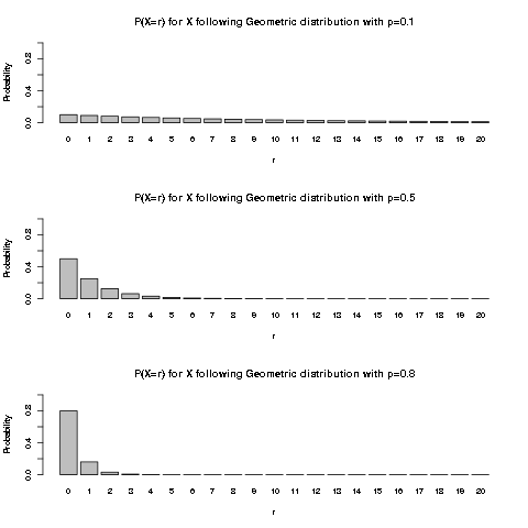
It is intuitively clear that with larger \(p\), i.e. higher probability of success, we would expect to get the first success earlier.
We remark that the Geometric distribution would be appropriate only if the independence assumption is plausible, i.e. a failure does not affect the probability of future success or failure; and that the Bernoulli trials are identically distributed, i.e. the probability of success does not change from trial to trial.
Expected value and variance
For calculating the expected value of \(X\) following Geometric distribution with parameter \(0 < p < 1\), we could have used the definition, i.e. \(E(X) = \sum_{r=1}^{\infty} {r P(X=r)}\), but the derivation needs differential calculus, so we just list it for completeness, and will not go through it in details.
\begin{align}
E(X) & = \sum_{r=0}^{\infty} {r P(X=r)} \\\
& = \sum_{r=1}^{\infty} {r (1-p)^{r}p} \\\
& = p(1-p) \sum_{r=1}^{\infty} {r (1-p)^{r-1}} \\\
& = p(1-p) \sum_{r=1}^{\infty} \left\{-\frac{d}{dp} {(1-p)^r} \right\} \\\
& = p(1-p) \frac{d}{dp} \left\{\sum_{r=1}^{\infty} {- {(1-p)^r}} \right\} \\\
& = p(1-p) \frac{d}{dp} \left\{1 - \frac{1}{1 - (1-p)} \right\} \\\
& = p(1-p) \frac{d}{dp} \left\{1 - \frac{1}{p} \right\} \\\
& = p(1-p) {\frac{1}{p^2}} \\\
& = \frac{1-p}{p}
\end{align}
Alternatively, we can use the memoryless property mentioned above to see what the expected value should be.
- Calculating expected value using memoryless property
By the memoryless property, if the first trial is a success, then
\\(X=0\\); if the first trial is a failure, then disregarding it, the
count to the first success still follows a Geometric distribution with
the same distribution. We therefore have

\begin{align}
X & = I\\{\text{success at first trial}\\}(0) + I\\{\text{failure at first trial}\\}(1 + X') \\\\\\
& = I\\{\text{failure at first trial}\\}(1 + X')
\end{align}

where \\(I\\{.\\}\\) is the indicator random variable, and \\(X'\\) is a random
variable that follows the same Geometric distribution as \\(X\\). Note
that since \\(1+X'\\) depends only on second and future trials,
\\(I\\{\text{failure at first trial}\\}\\) and \\((1 + X')\\) are independent.

Then by expected value of independent random variables, we must have

\begin{align}
E(X) & = E[I\\{\text{failure at first trial}\\}(1 + X')] \\\\\\
& = E[I\\{\text{failure at first trial}\\}] E[(1 + X')] \\\\\\
& = (1-p)(1 + E(X')) \\\\\\
& = (1-p)(1 + E(X))
\end{align}

where the expected value of an indicator variable is the probability
of its event, and that \\(E(X') = E(X)\\) because \\(X\\) and \\(X'\\) have the
same distribution.

Then we rearrange the terms to put \\(E(X)\\) on the left side, we have:

\begin{align}
E(X) & = (1-p)(1 + E(X)) \\\\\\
E(X) - (1-p)E(X) & = (1-p) \\\\\\
p E(X) & = 1 - p \\\\\\
E(X) & = \frac{1-p}{p}
\end{align}

We therefore see that if \\(E(X)\\) exists, it must be \\(\frac{1-p}{p}\\).

The interpretation of the expected value is simple, if the success
probability of each trial is \\(p\\), then we expect to need
\\(\frac{1-p}{p} = \frac{1}{p}-1\\) failures to get a success, so with a
higher probability of success, we expect smaller number of failures
until a success. E.g. if \\(p=0.1\\), the expected number of failures is
\\(\frac{1-0.1}{0.1} = 9\\) until a success.

We emphasize one interesting aspect of the expected value related to
the memoryless property. Before seeing any trials, we expect to need
\\(\frac{1-p}{p}\\) failures until the first success. But given that we
have just observed a failure, we still expect to need \\(\frac{1-p}{p}\\)
future failures until the first success. That is, for the \\(p=0.1\\)
example, if we observed a failure, we would still expect to need 9
future trials until a success, not 8, due to the memoryless property!
- Calculating the variance
For the variance, we again try to use the memoryless property, and the
formula \\(Var(X) = E(X^2) - [E(X)]^2\\). We note that \\(X^2 =
I\\{\text{failure at first trial}\\}(1 + X')^2\\), then we first calculate
\\(E(X^2)\\) as:

\begin{align}
E(X^2) & = E[I\\{\text{failure at first trial}\\}(1 + X')^2] \\\\\\
& = E[I\\{\text{failure at first trial}\\}] E[1 + 2X' + X'^2] \\\\\\
& = (1-p)(1 + 2 E(X') + E(X'^2)) \\\\\\
& = (1-p)(1 + \frac{2(1-p)}{p} + E(X^2)) \\\\\\
& = (1-p) + \frac{2(1-p)^2}{p} + (1-p)E(X^2)
\end{align}

Then rearrange the terms, we have

\begin{align}
(1 - (1-p))E(X^2) & = (1-p) + \frac{2(1-p)^2}{p} \\\\\\
         p E(X^2) & = (1-p) + \frac{2(1-p)^2}{p} \\\\\\
           E(X^2) & = \frac{1-p}{p} + \frac{2(1-p)^2}{p^2} \\\\\\
\end{align}

Then we calculate \\(Var(X)\\) as:

\begin{align}
Var(X) & = E(X^2) - [E(X)]^2 \\\\\\
& = \frac{1-p}{p} + \frac{2(1-p)^2}{p^2} - \left[\frac{1-p}{p} \right]^2 \\\\\\
& = \frac{1-p}{p} + \frac{(1-p)^2}{p^2} \\\\\\
& = \frac{p(1-p) + (1-p)^2}{p^2} \\\\\\
& = \frac{1-p}{p^2} \\\\\\
\end{align}

So a higher probability of success results in a lower variance.
Negative Binomial Distribution
We are still using the framework of independent Bernoulli trials with parameter \(0 < p < 1\), while in Geometric distribution we count the number of failures to get the first success, what if we consider the number of failures \(X\) to get \(k\) successes, for \(k > 0\)?. For example, if we count the number of “tails” before we get 3 heads, what is the distribution of the count? Such an \(X\) is said to follow the Negative binomial distribution, with parameters \(k > 0\) and \(0 < p < 1\), and we would write \(X \sim NB(k, p)\). Again we remark that there are alternative definitions of the Negative binomial distribution:
- some may count the number of trials until \(k\) successes.
- some may interchange the role of success and failure, i.e. count the number of successes until \(k\) failures, or count the number of trials until \(k\) failures.
Therefore, when you encounter the term “Negative binomial distribution”, it is important to know the exact definition used, to avoid confusion. To be consistent with the convention for Geometric distribution, we would stick to the definition of counting the number of failures until \(k\) successes.
We immediately see that \(X \geq 0\), i.e. we may get 0 failures if the first \(k\) trials are all successes, and again \(X\) has no upper bound. It is also intuitively clear that \(X\) can be written as the sum of \(k\) mutually independent random variables following Geometric distribution with parameter \(p\), i.e. \(X = X_1 + X_2 + \ldots + X_k\), where the \(\{X_i\}\) are mutually independent and all follow the same Geometric distribution: to count the failures to get \(k\) successes, we count the failures to get the first success, then the second, and so on, until the \(k\) th success, then add the counts together. Moreover, the Geometric distribution is a special case of the Negative binomial distribution where \(k=1\).
Probability mass function for Negative binomial distribution
What should be \(P(X=r)\) for \(X \sim NB(k,p)\)? Before we figure out the general formula, let’s first consider a small concrete example of \(P(X'=2)\) for \(X' \sim NB(3,p)\), to get an intuitive idea.
We list out the possibilities of needing 2 failures to get 3 successes (written as 1 below), since there are 2 failures and 3 successes, there are 5 trials:
| Trial 1 | Trial 2 | Trial 3 | Trial 4 | Trial 5 | Probability |
|---|---|---|---|---|---|
| 1 | 1 | 0 | 0 | 1 | \(pp(1-p)(1-p)p = p^3(1-p)^2\) |
| 1 | 0 | 1 | 0 | 1 | \(p(1-p)p(1-p)p = p^3(1-p)^2\) |
| 1 | 0 | 0 | 1 | 1 | \(p(1-p)(1-p)pp = p^3(1-p)^2\) |
| 0 | 1 | 1 | 0 | 1 | \((1-p)pp(1-p)p = p^3(1-p)^2\) |
| 0 | 1 | 0 | 1 | 1 | \((1-p)p(1-p)pp = p^3(1-p)^2\) |
| 0 | 0 | 1 | 1 | 1 | \((1-p)(1-p)ppp = p^3(1-p)^2\) |
We note a few things:
- trial 5 is always a success, since we stop counting as soon as we get 3 successes.
- in each combination, there are 3 successes and 2 failures, so the probability is the same: \(p^3(1-p)^2\).
- this is similar to the Binomial distribution we considered above, since each combination has the same probability, we need only figure out the number of combinations to get the desired probability.
Since trial 5 is always a success, the 2 failures can appear in any two of trial 1 to 4, so there are \(C_2^4 = \frac{4!}{2!2!} = 6\) possible combinations. Therefore, \(P(X'=2) = C_2^4 {p^3(1-p)^2}\).
We can use the same idea for the general case. To determine \(P(X=r)\) for \(X \sim NB(k,p)\), since we stopped counting at trial \(r+k\), it must be the \(k\) th success, and the \(r\) failures can appear in any of the previous \(r+k-1\) trials, so there are \(C_{r}^{r+k-1}\) combinations, and each has the same probability of \(p^k(1-p)^{r}\) because there are \(k\) successes and \(r\) failures. We therefore have figured out the pmf of the Negative binomial distribution as:
\begin{equation} P(X=r) = C_{r}^{r+k-1} {p^{k}(1-p)^{r}} \end{equation}
We plot the first few values of the pmf of the Negative binomial distribution for some values of \(k\) and \(p\):
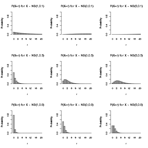
We see that for larger success probability \(p\), the probability is more concentrated on the smaller values of \(X\), because it would be easier to get the first \(k\) successes. Also for smaller \(p\), the distribution is more spread out. For larger number of successes \(k\), the distribution will move more to the right, because intuitively more failures would be encountered to accumulate a larger number of successes, and the effect is greater for smaller \(p\).
We briefly note that in R, the “negative binomial distribution” (dnbinom) allows \(k\) to take non-integer value, because it is in fact a more general distribution, where the Geometric distribution, the Negative binomial distribution we introduced above, and the Poisson distribution to be introduced below are special cases.
Expected value and variance
Recall that \(X \sim NB(k,p)\) could be written as a sum of \(k\) i.i.d. random variables following Geometric distribution, i.e. \(X = \sum_{i=1}^k {X_i}\), where \(\{X_i\}\) are mutually independent, and each has the same Geometric distribution with parameter \(p\). By the linearity of expected value, and the independence of the random variables, it is easy to figure out the expected value and variance of \(X\), as follows:
\begin{align}
E(X) & = E \left(\sum_{i=1}^k {X_i} \right) \\\
& = \sum_{i=1}^k {E(X_i)} \\\
& = \sum_{i=1}^k {\frac{1-p}{p}} \\\
& = \frac{k(1-p)}{p}
\end{align}
and
\begin{align}
Var(X) & = Var \left(\sum_{i=1}^k {X_i} \right) \\\
& = \sum_{i=1}^k {Var(X_i)} \\\
& = \sum_{i=1}^k {\frac{1-p}{p^2}} \\\
& = \frac{k(1-p)}{p^2}
\end{align}
Poisson Distribution
Law of rare events
Poisson is a distribution that models the count of events over “an interval” (an “exposure”), which could be a length (e.g. a segment of an undersea cable), an area, a volume, a time duration (e.g. a year).
Poisson distribution is used to model the counts of events satisfying the law of rare events, where the assumptions are:
- the count is the number of events in “an interval”
- the occurrences of the events in non-overlapping sub-intervals are independent
- the average rate of events is constant
- two events do not occur at the exact same point in the interval, at an infinitely small sub-interval, either exactly one event occurs, or no event occurs
Probability mass function for Poisson distribution
With the assumptions of law of rare events, we outline the derivation of the pmf of Poisson distribution. Let \(X\) be the counts of events over an interval, with the constant event rate being \(\lambda\). Suppose we divide the interval into \(N\) non-overlapping sub-intervals (with equal lengths). By assumption, with sufficiently fine sub-intervals, the counts of event in sub-intervals are independent, and each is either 0 or 1, so the total counts over the sub-intervals follows \(B(N,p)\) for some probability \(p\) (which depends on \(N\)). Also, by the assumption of constant event rate, we have \(\lim_{N \to \infty} {Np} = \lambda\).
Then we have
\begin{align}
P(X=r) & = C_r^N {p^r (1-p)^{N-r}} \\\
& = \frac{N!}{r!(N-r)!} {p^r (1-p)^{N-r}} \\\
& = \frac{N!}{r!(N-r)!} {{\left(\frac{Np}{N}\right)}^r {\left( 1- \frac{Np}{N} \right)}^{N-r}} \\\
& = \frac{N!}{(N-r)! N^r} {\frac{(Np)^r}{r!} {\left( 1- \frac{Np}{N} \right)}^N {\left( 1- \frac{Np}{N} \right)}^{-r}} \\\
\end{align}
Now as \(N \to \infty\), we check what each of the terms converge to:
First for \(\frac{N!}{(N-r)! N^r}\)
\begin{align}
\frac{N!}{(N-r)! N^r} & = \frac{N(N-1)(N-2)\ldots (N-r+1)}{N^r} \\\
& = \frac{N}{N} \frac{N-1}{N} \frac{N-2}{N} \ldots \frac{N-r+1}{N} \\\
& = \left(1 \right) \left(1-\frac{1}{N} \right) \left(1-\frac{2}{N} \right) \ldots \left(1-\frac{r-1}{N} \right) \\\
& \to 1 \text{ as } r \text{ is fixed}
\end{align}
Then for \(\frac{(Np)^r}{r!}\)
\begin{align} \frac{(Np)^r}{r!} \to \frac{\lambda^r}{r!} \end{align}
Then for \({\left( 1- \frac{Np}{N} \right)}^N\)
\begin{align}
{\left( 1- \frac{Np}{N} \right)}^N & \to e^{-\lambda} \\\
& \text{because } Np \to \lambda \text{ and } \\\
& {\left( 1 - \frac{x}{n} \right)}^n \to e^{-x} \text{ as } n \to \infty
\end{align}
Lastly for \({\left( 1- \frac{Np}{N} \right)}^{-r}\)
\begin{align}
{\left( 1- \frac{Np}{N} \right)}^{-r} & \to 1 \\\
& \text{because } Np \to \lambda \text{, so } \frac{Np}{N} \to 0
\end{align}
We therefore see that as \(N \to \infty\)
\begin{align}
P(X=r) & \to (1)\frac{\lambda^r}{r!} e^{-\lambda} (1) \\\
& = \frac{e^{-\lambda} \lambda^r}{r!}
\end{align}
which is the pmf of the Poisson distribution, with parameter \(\lambda > 0\).
We sometimes write \(X \sim Pois(\lambda)\) to denote that \(X\) follows a Poisson distribution with parameter \(\lambda > 0\). Note that \(\lambda\) need not be an integer. Also note that \(X\) can take any non-negative integers, again without upper bound, i.e. \(P(X=r) > 0\) for any integer \(r \geq 0\).
Also, we check that the probabilities sum to 1:
\begin{align}
\sum_{r=0}^{\infty} {P(X=r)} & = \sum_{r=0}^{\infty} {\frac{e^{-\lambda} \lambda^r}{r!}} \\\
& = e^{-\lambda} \sum_{r=0}^{\infty} {\frac{\lambda^r}{r!}} \\\
& = e^{-\lambda} e^{\lambda} \\\
& = 1 \\\
& \text{ by the power series } \sum_{r=0}^{\infty} {\frac{x^r}{r!}} = e^{x}
\end{align}
We briefly mention a few properties of Poisson distribution:
- If \(X \sim Pois(\lambda)\) counts the events with constant rate \(\lambda\) on an interval with certain length (or size) \(L\), then the count on the interval with length \(kL\) for \(k > 0\) would follow \(Pois(k \lambda)\). In other words, with constant rate, the counts on different sizes of the interval also follow Poisson distribution, with the parameter scaled by the length of the interval.
- Sum of independent Poisson random variables also follows Poisson distribution, where the parameter is the sum of the parameters, i.e. if \(X_i \sim Pois(\lambda_i)\), then \(\sum_{i} {X_i} \sim Pois(\sum_i \lambda_i)\). Note that the \(\lambda\)’s may not be equal.
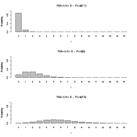
We plot the first few values of pmf of Poisson distribution for a few \(\lambda\) values:
Expected value and variance
In the above derivation, we derive the pmf of Poisson distribution from \(B(N,p)\) as \(N \to \infty\). For each \(N\), the expected value of the total count is \(Np \to \lambda\), and the variance is \(Np(1-p) = Np(1- \frac{Np}{N}) \to \lambda\). It is a reasonable guess that both the expected value and variance of \(Pois(\lambda)\) are \(\lambda\). This is indeed the case, we just quickly show it from the definition.
\begin{align}
E(X) & = \sum_{r=0}^{\infty} {r P(X=r)} \\\
& = \sum_{r=0}^{\infty} {r \frac{e^{-\lambda} \lambda^r}{r!}} \\\
& = \sum_{r=1}^{\infty} {r \frac{e^{-\lambda} \lambda^r}{r!}} \text{ as zero times anything is zero} \\\
& = \lambda e^{-\lambda} \sum_{r-1=0}^{\infty} {\frac{\lambda^{r-1}}{(r-1)!}} \\\
& = \lambda e^{-\lambda} e^{\lambda} \text{, again by the power series } \sum_{u=0}^{\infty} {\frac{x^u}{u!}} = e^{x} \\\
& = \lambda
\end{align}
For variance, we first calculate \(E(X^2)\):
\begin{align}
E(X^2) & = E[X(X-1) + X] \\\
& = E[X(X-1)] + E(X) \\\
& = E(X) + \sum_{r=0}^{\infty} {r(r-1) P(X=r)} \\\
& = E(X) + \sum_{r=2}^{\infty} {r(r-1) \frac{e^{-\lambda} \lambda^r}{r!}} \text{ as } r(r-1)=0 \text{ for } r=0 \text{ or } r=1\\\
& = E(X) + \lambda^2 e^{-\lambda} \sum_{r=2}^{\infty} {\frac{\lambda^{r-2}}{(r-2)!}} \\\
& = E(X) + \lambda^2 e^{-\lambda} \sum_{r-2=0}^{\infty} {\frac{\lambda^{r-2}}{(r-2)!}} \\\
& = E(X) + \lambda^2 e^{-\lambda} e^{\lambda} \text{, again by the power series } \sum_{u=0}^{\infty} {\frac{x^u}{u!}} = e^{x} \\\
& = E(X) + \lambda^2 \\\
& = \lambda + \lambda^2
\end{align}
Then we have
\begin{align}
Var(X) & = E(X^2) - [E(X)]^2 \\\
& = \lambda + \lambda^2 - \lambda^2 \\\
& = \lambda
\end{align}
Example: Number of defects in undersea cable
One simple example is to model the number of defects in undersea cable, where we may assume a constant rate \(\lambda\) of defects per 1km, then over any segment of cable of length \(L\) km, the distribution of the count is \(Pois(L \lambda)\).
Example: Hospital benefit claims over a year
An example in insurance is the number of hospital benefit claims over a year with an assumed rate \(\lambda\), where one policy may have zero or more claims over a year. The claim count of each policy can be modeled as \(Pois(\lambda_i)\). If we are only counting the claims over a period of 9 months, then the distribution would be \(Pois(\frac{9}{12} \lambda_i)\). If we are interested in the total claims counts of \(n\) policies over one calendar year, assuming the claims of the different policies are independent, the distribution is \(Pois(\sum_{i=1}^n \lambda_i t_i)\), where \(t_i\) is the exposure period of the \(i\) th policy. For example, if a policy is issued in the middle of the year, its exposure would only be 0.5 year till the end of the calendar year. We remark that the \(\lambda_i\) ’s need not be the same for all \(i\), but can be different for each policy, if we wish to model the rate \(\lambda_i\) ’s using covariates associated with the \(i\) th policy. We will revisit this idea in a future post when we discuss the Generalized Linear Model.
Summary
In this post, we have looked at some common discrete distributions:
- Discrete uniform distribution: the probabilities of each of the \(k\) finite possible values have the same value \(\frac{1}{k}\)
- Bernoulli distribution: only two possible values, the value 1 (often called a “success”) with probability \(p \geq 0\), and the value 0 (often called a “failure”) with probability \(1-p\).
- Binomial distribution: the sum of \(n\) i.i.d. Bernoulli random variables, with pmf \(P(X=r) = C_r^n p^r (1-p)^{n-r}\).
- Geometric distribution: the number of Bernoulli failures until the first success, in a series of i.i.d. Bernoulli trials, with pmf \(P(X=r) = (1-p)^{r}p\).
- Negative binomial distribution: the number of Bernoulli failures until \(k\) successes, in a series of i.i.d. Bernoulli trials, with pmf \(P(X=r) = C_{r}^{r+k-1} {p^{k}(1-p)^{r}}\).
- Poisson distribution: the count of events over an interval with constant event rate \(\lambda\), where the count follows the law of rare events, with pmf \(P(X=r) = \frac{e^{-\lambda} \lambda^r}{r!}\).
For completeness, we have also derived that the variance of a sum of independent random variables is the sum of the variances. We also briefly mentioned the covariance of two numerical random variables.
We will turn our focus to continuous distribution in a future post, before we turn to look at maximum likelihood estimation.
Author Peter Lo
LastMod 2019-06-16